ХвЖӘҪМіМОв¶чҙп»ъЖчС§П°Б·П°:SVMЦ§іЦПтБҝ»ъРҙөГәЬКөУГЈ¬ПЈНыДЬ°пөҪДъЎЈ
1 Support Vector Machines1.1 Example Dataset 1%matplotlib inlineimport numpy as npimport pandas as pdimport matplotlib.pyplot as pltimport seaborn as sbfrom scipy.io import loadmatfrom sklearn import svm ҙу¶аКэSVMөДҝв»бЧФ¶Ҝ°пДгМнјУ¶оНвөДМШХчX₀ТСҫӯҰИ₀Ј¬ЛщТФОЮРиКЦ¶ҜМнјУ mat = loadmat('./data/ex6data1.mat')print(mat.keys())# dict_keys(['__header__', '__version__', '__globals__', 'X', 'y'])X = mat['X']y = mat['y']def plotData(X, y): plt.figure(figsize=(8,5)) plt.scatter(X[:,0], X[:,1], c=y.flatten(), cmap='rainbow') plt.xlabel('X1') plt.ylabel('X2') plt.legend() plotData(X, y)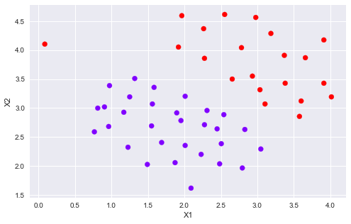
def plotBoundary(clf, X): '''plot decision bondary''' x_min, x_max = X[:,0].min()*1.2, X[:,0].max()*1.1 y_min, y_max = X[:,1].min()*1.1,X[:,1].max()*1.1 xx, yy = np.meshgrid(np.linspace(x_min, x_max, 500), np.linspace(y_min, y_max, 500)) Z = clf.predict(np.c_[xx.ravel(), yy.ravel()]) Z = Z.reshape(xx.shape) plt.contour(xx, yy, Z) models = [svm.SVC(C, kernel='linear') for C in [1, 100]]clfs = [model.fit(X, y.ravel()) for model in models] title = ['SVM Decision Boundary with C = {} (Example Dataset 1'.format(C) for C in [1, 100]]for model,title in zip(clfs,title): plt.figure(figsize=(8,5)) plotData(X, y) plotBoundary(model, X) plt.title(title)
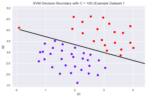
ҝЙТФҙУЙПНјҝҙөҪЈ¬өұCұИҪПРЎКұДЈРН¶ФОу·ЦАаөДіН·ЈФцҙуЈ¬ұИҪПСПёсЈ¬Оу·ЦАаЙЩЈ¬јдёфұИҪППБХӯЎЈ өұCұИҪПҙуКұДЈРН¶ФОу·ЦАаөДіН·ЈФцҙуЈ¬ұИҪПҝнЛЙЈ¬ФКРнТ»¶ЁөДОу·ЦАаҙжФЪЈ¬јдёфҪПҙуЎЈ 1.2 SVM with Gaussian KernelsХвІҝ·ЦЈ¬К№УГSVMЧц·ЗПЯРФ·ЦАаЎЈОТГЗҪ«К№УГёЯЛ№әЛәҜКэЎЈ ОӘБЛУГSVMХТіцТ»ёц·ЗПЯРФөДҫцІЯұЯҪзЈ¬ОТГЗКЧПИТӘКөПЦёЯЛ№әЛәҜКэЎЈОТҝЙТФ°СёЯЛ№әЛәҜКэПлПуіЙТ»ёцПаЛЖ¶ИәҜКэЈ¬УГАҙІвБҝТ»¶ФСщұҫөДҫаАлЈ¬(x ⁽ ʲ ⁾,y ⁽ ⁱ ⁾) 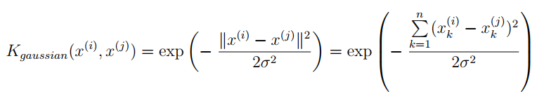
ХвАпОТГЗУГsklearnЧФҙшөДsvmЦРөДәЛәҜКэјҙҝЙЎЈ 1.2.1 Gaussian Kerneldef gaussKernel(x1, x2, sigma): return np.exp(- ((x1 - x2) ** 2).sum() / (2 * sigma ** 2))gaussKernel(np.array([1, 2, 1]),np.array([0, 4, -1]), 2.) # 0.32465246735834974 1.2.2 Example Dataset 2mat = loadmat('./data/ex6data2.mat')X2 = mat['X']y2 = mat['y']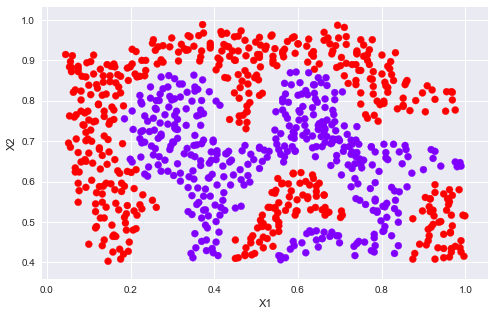
sigma = 0.1gamma = np.power(sigma,-2.)/2clf = svm.SVC(C=1, kernel='rbf', gamma=gamma)modle = clf.fit(X2, y2.flatten())plotData(X2, y2)plotBoundary(modle, X2) 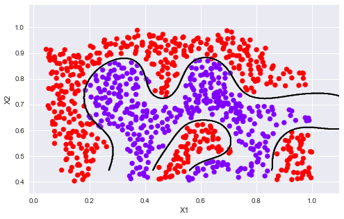
1.2.3 Example Dataset 3mat3 = loadmat('data/ex6data3.mat')X3, y3 = mat3['X'], mat3['y']Xval, yval = mat3['Xval'], mat3['yval']plotData(X3, y3)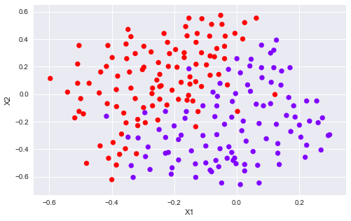
Cvalues = (0.01, 0.03, 0.1, 0.3, 1., 3., 10., 30.)sigmavalues = Cvaluesbest_pair, best_score = (0, 0), 0for C in Cvalues: for sigma in sigmavalues: gamma = np.power(sigma,-2.)/2 model = svm.SVC(C=C,kernel='rbf',gamma=gamma) model.fit(X3, y3.flatten()) this_score = model.score(Xval, yval) if this_score > best_score: best_score = this_score best_pair = (C, sigma)print('best_pair={}, best_score={}'.format(best_pair, best_score))# best_pair=(1.0, 0.1), best_score=0.965model = svm.SVC(C=1., kernel='rbf', gamma = np.power(.1, -2.)/2)model.fit(X3, y3.flatten())plotData(X3, y3)plotBoundary(model, X3) 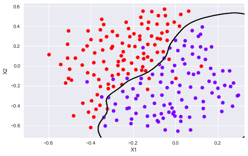
# ХвОТөДТ»ёцБ·П°»ӯНјөДЈ¬әНЧчТөОЮ№ШЈ¬ёшёц»ӯНјөДІОҝјЎЈimport numpy as npimport matplotlib.pyplot as pltfrom sklearn import svm# we create 40 separable pointsnp.random.seed(0)X = np.array([[3,3],[4,3],[1,1]])Y = np.array([1,1,-1])# fit the modelclf = svm.SVC(kernel='linear')clf.fit(X, Y)# get the separating hyperplanew = clf.coef_[0]a = -w[0] / w[1]xx = np.linspace(-5, 5)yy = a * xx - (clf.intercept_[0]) / w[1]# plot the parallels to the separating hyperplane that pass through the# support vectorsb = clf.support_vectors_[0]yy_down = a * xx + (b[1] - a * b[0])b = clf.support_vectors_[-1]yy_up = a * xx + (b[1] - a * b[0])# plot the line, the points, and the nearest vectors to the planeplt.figure(figsize=(8,5))plt.plot(xx, yy, 'k-')plt.plot(xx, yy_down, 'k--')plt.plot(xx, yy_up, 'k--')# ИҰіцЦ§іЦПтБҝplt.scatter(clf.support_vectors_[:, 0], clf.support_vectors_[:, 1], s=150, facecolors='none', edgecolors='k', linewidths=1.5)plt.scatter(X[:, 0], X[:, 1], c=Y, cmap=plt.cm.rainbow)plt.axis('tight')plt.show()print(clf.decision_function(X))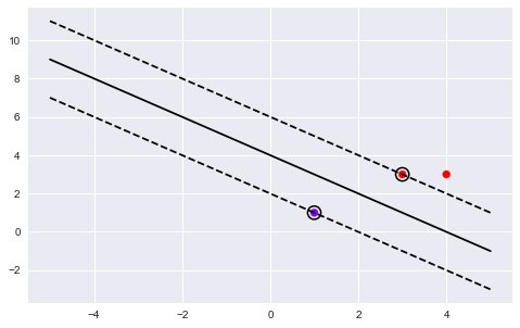
2 Spam Classification2.1 Preprocessing EmailsХвІҝ·ЦУГSVMҪЁБўТ»ёцА¬»шУКјю·ЦАаЖчЎЈДгРиТӘҪ«ГҝёцemailұдіЙТ»ёцnО¬өДМШХчПтБҝЈ¬Хвёц·ЦАаЖчҪ«ЕР¶Пёш¶ЁТ»ёцУКјюxКЗА¬»шУКјю(y=1)»тІ»КЗА¬»шУКјю(y=0)ЎЈ take a look at examples from the dataset with open('data/emailSample1.txt', 'r') as f: email = f.read() print(email)> Anyone knows how much it costs to host a web portal ?>Well, it depends on how many visitors you're expecting.This can be anywhere from less than 10 bucks a month to a couple of $100. You should checkout http://www.rackspace.com/ or perhaps Amazon EC2 if youre running something big..To unsubscribe yourself from this mailing list, send an email to:groupname-unsubscribe@egroups.com ҝЙТФҝҙөҪЈ¬УКјюДЪИЭ°ьә¬ a URL, an email address(at the end), numbers, and dollar amounts. әЬ¶аУКјю¶ј»б°ьә¬ХвР©ФӘЛШЈ¬ө«КЗГҝ·вУКјюөДҫЯМеДЪИЭҝЙДЬ»бІ»Т»СщЎЈТтҙЛЈ¬ҙҰАнУКјюҫӯіЈІЙУГөД·Ҫ·ЁКЗұкЧј»ҜХвР©КэҫЭЈ¬°СЛщУРURLөұЧчТ»СщЈ¬ЛщУРКэЧЦҝҙЧчТ»СщЎЈ АэИзЈ¬ОТГЗУГОЁТ»өДТ»ёцЧЦ·ыҙ®Ў®httpaddr'АҙМж»»ЛщУРөДURLЈ¬АҙұнКҫУКјю°ьә¬URLЈ¬¶шІ»ТӘЗуҫЯМеөДURLДЪИЭЎЈХвНЁіЈ»бМбёЯА¬»шУКјю·ЦАаЖчөДРФДЬЈ¬ТтОӘА¬»шУКјю·ўЛНХЯНЁіЈ»бЛж»ъ»ҜURLЈ¬ТтҙЛФЪРВөДА¬»шУКјюЦРФЩҙОҝҙөҪИОәОМШ¶ЁURLөДјёВК·ЗіЈРЎЎЈ ОТГЗҝЙТФЧцИзПВҙҰАнЈә 1. Lower-casing: °СХы·вУКјюЧӘ»ҜОӘРЎРҙЎЈ 2. Stripping HTML: ТЖіэЛщУРHTMLұкЗ©Ј¬Ц»ұЈБфДЪИЭЎЈ 3. Normalizing URLs: Ҫ«ЛщУРөДURLМж»»ОӘЧЦ·ыҙ® Ў°httpaddrЎұ. 4. Normalizing Email Addresses: ЛщУРөДөШЦ·Мж»»ОӘ Ў°emailaddrЎұ 5. Normalizing Dollars: ЛщУРdollar·ыәЕ($)Мж»»ОӘЎ°dollarЎұ. 6. Normalizing Numbers: ЛщУРКэЧЦМж»»ОӘЎ°numberЎұ 7. Word Stemming(ҙКёЙМбИЎ): Ҫ«ЛщУРөҘҙК»№ФӯОӘҙКФҙЎЈАэИзЈ¬Ў°discountЎұ, Ў°discountsЎұ, Ў°discountedЎұ and Ў°discountingЎұ¶јМж»»ОӘЎ°discountЎұЎЈ 8. Removal of non-words: ТЖіэЛщУР·ЗОДЧЦАаРНЈ¬ЛщУРөДҝХёс(tabs, newlines, spaces)өчХыОӘТ»ёцҝХёс. %matplotlib inlineimport numpy as npimport matplotlib.pyplot as pltfrom scipy.io import loadmatfrom sklearn import svmimport re #regular expression for e-mail processing# ХвКЗТ»ёцҝЙУГөДУўОД·ЦҙКЛг·Ё(Porter stemmer)from stemming.porter2 import stem# ХвёцУўОДЛг·ЁЛЖәхёь·ыәПЧчТөАпГжЛщУГөДҙъВлЈ¬УлЙПГжР§№ыІоІ»¶аimport nltk, nltk.stem.porter def processEmail(email): """ЧціэБЛWord StemmingәНRemoval of non-wordsөДЛщУРҙҰАн""" email = email.lower() email = re.sub('<[^<>]>', ' ', email) # ЖҘЕд<ҝӘН·Ј¬И»әуЛщУРІ»КЗ< ,> өДДЪИЭЈ¬ЦӘөА>ҪбОІЈ¬ПаөұУЪЖҘЕд<...> email = re.sub('(http|https)://[^/s]*', 'httpaddr', email ) # ЖҘЕд//әуГжІ»КЗҝХ°ЧЧЦ·ыөДДЪИЭЈ¬УцөҪҝХ°ЧЧЦ·ыФтНЈЦ№ email = re.sub('[^/s]+@[^/s]+', 'emailaddr', email) email = re.sub('[/$]+', 'dollar', email) email = re.sub('[/d]+', 'number', email) return emailҪУПВАҙҫНКЗМбИЎҙКёЙЈ¬ТФј°ИҘіэ·ЗЧЦ·ыДЪИЭЎЈ def email2TokenList(email): """ФӨҙҰАнКэҫЭЈ¬·ө»ШТ»ёцёЙҫ»өДөҘҙКБРұн""" # I'll use the NLTK stemmer because it more accurately duplicates the # performance of the OCTAVE implementation in the assignment stemmer = nltk.stem.porter.PorterStemmer() email = preProcess(email) # Ҫ«УКјю·ЦёоОӘөҘёцөҘҙКЈ¬re.split() ҝЙТФЙиЦГ¶аЦЦ·Цёф·ы tokens = re.split('[ /@/$///#/./-/:/&/*/+/=/[/]/?/!/(/)/{/}/,/'/"/>/_/</;/%]', email) # ұйАъГҝёц·ЦёоіцАҙөДДЪИЭ tokenlist = [] for token in tokens: # ЙҫіэИОәО·ЗЧЦДёКэЧЦөДЧЦ·ы token = re.sub('[^a-zA-Z0-9]', '', token); # Use the Porter stemmer to МбИЎҙКёщ stemmed = stemmer.stem(token) # ИҘіэҝХЧЦ·ыҙ®Ў®'Ј¬АпГжІ»ә¬ИОәОЧЦ·ы if not len(token): continue tokenlist.append(stemmed) return tokenlist 2.1.1 Vocabulary List(ҙК»гұн)ФЪ¶ФУКјюҪшРРФӨҙҰАнЦ®әуЈ¬ОТГЗУРТ»ёцҙҰАнәуөДөҘҙКБРұнЎЈПВТ»ІҪКЗСЎФсОТГЗПлФЪ·ЦАаЖчЦРК№УГДДР©ҙКЈ¬ОТГЗРиТӘИҘіэДДР©ҙКЎЈ ОТГЗУРТ»ёцҙК»гұнvocab.txtЈ¬АпГжҙжҙўБЛФЪКөјКЦРҫӯіЈК№УГөДөҘҙКЈ¬№І1899ёцЎЈ ОТГЗТӘЛгіцҙҰАнәуөДemailЦРә¬УР¶аЙЩvocab.txtЦРөДөҘҙКЈ¬Іў·ө»ШФЪvocab.txtЦРөДindexЈ¬ХвҫНОТГЗПлТӘөДСөБ·өҘҙКөДЛчТэЎЈ def email2VocabIndices(email, vocab): """МбИЎҙжФЪөҘҙКөДЛчТэ""" token = email2TokenList(email) index = [i for i in range(len(vocab)) if vocab[i] in token ] return index 2.2 Extracting Features from Emailsdef email2FeatureVector(email): """ Ҫ«emailЧӘ»ҜОӘҙКПтБҝЈ¬nКЗvocabөДіӨ¶ИЎЈҙжФЪөҘҙКөДПаУҰО»ЦГөДЦөЦГОӘ1Ј¬ЖдУаОӘ0 """ df = pd.read_table('data/vocab.txt',names=['words']) vocab = df.as_matrix() # return array vector = np.zeros(len(vocab)) # init vector vocab_indices = email2VocabIndices(email, vocab) # ·ө»Шә¬УРөҘҙКөДЛчТэ # Ҫ«УРөҘҙКөДЛчТэЦГОӘ1 for i in vocab_indices: vector[i] = 1 return vectorvector = email2FeatureVector(email)print('length of vector = {}/nnum of non-zero = {}'.format(len(vector), int(vector.sum())))length of vector = 1899num of non-zero = 45 2.3 Training SVM for Spam Classification¶БИЎТСҫӯСөМбИЎәГөДМШХчПтБҝТФј°ПаУҰөДұкЗ©ЎЈ·ЦСөБ·јҜәНІвКФјҜЎЈ # Training setmat1 = loadmat('data/spamTrain.mat')X, y = mat1['X'], mat1['y']# Test setmat2 = scipy.io.loadmat('data/spamTest.mat')Xtest, ytest = mat2['Xtest'], mat2['ytest']clf = svm.SVC(C=0.1, kernel='linear')clf.fit(X, y) 2.4 Top Predictors for SpampredTrain = clf.score(X, y)predTest = clf.score(Xtest, ytest)predTrain, predTest өҪҙЛХвЖӘ№ШУЪ»ъЖчС§П°SVMЦ§іЦПтБҝ»ъөДБ·П°ОДХВҫНҪйЙЬөҪХвБЛ,ёь¶аПа№Ш»ъЖчС§П°ДЪИЭЗлЛСЛч51zixue.netТФЗ°өДОДХВ»тјМРшдҜААПВГжөДПа№ШОДХВЈ¬ПЈНыҙујТТФәу¶а¶аЦ§іЦ51zixue.netЈЎ
Python Ҫвҫцlogging№ҰДЬК№УГ№эіМЦРУцөҪөДТ»ёцОКМв
pythonАп¶БРҙexcelөИКэҫЭОДјюөД6ЦЦіЈУГ·ҪКҪ(РЎҪб) |


